
Simple Linear Regression
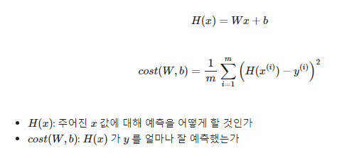
Data Definition
dataset : hours(x) , points(y)
데이터는 torch.tensor의 형태를 띄고 있다.
| Hours(x) | Points(y) |
| 1 | 1 |
| 2 | 2 |
| 3 | 3 |
x_train = torch.FloatTensor([[1], [2], [3]])
y_train = torch.FloatTensor([[1], [2], [3]])
print(x_train)
print(x_train.shape)

print('-------------------')

print(y_train)
print(y_train.shape)

##################output###################

tensor([[1.],
        [2.],
        [3.]])
torch.Size([3, 1])
-------------------
tensor([[1.],
        [2.],
        [3.]])
torch.Size([3, 1])
Hypothesis 초기화 및 구현

Weight와 bias를 정의 해야한다.
W = torch.zeros(1, requires_grad = True)
b = torch.zeros(1, requires_grad = True)
hypothesis = x_train * W + b
weight와 bias를 0으로 초기화한다. 처음에 어떤 input을 받아도 항상 output을 0이라고 예측한다.
w와 b를 학습 시키는 것이 목적이므로 requires_grad를 true라고 명시한다.
requires_grad를 true로 설정하면 연산을 추적한다.
Cost (loss 측정)
MSE로 loss를 측정한다.
#cost
print(hypothesis - y_train)

#torch.mean으로 평균 계산
mean_val = (hypothesis - y_train) ** 2
print((hypothesis - y_train) ** 2)

cost = torch.mean(mean_val)
print(cost)

##################output###################

tensor([[-1.],
        [-2.],
        [-3.]], grad_fn=<SubBackward0>)
tensor([[1.],
        [4.],
        [9.]], grad_fn=<PowBackward0>)
tensor(4.6667, grad_fn=<MeanBackward0>)
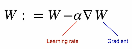
이제 계산한 loss를 바탕으로 loss 줄이는 최적화가 필요하다.
Optimizer 정의 (Gradient Descent)
optimizer = optim.SGD([W, b], lr = 0.01)
optimizer.zero_grad()
cost.backward()
optimizer.step()
torch.optim 라이브러리를 사용한다.
학습시킬 변수를 list로 만들어 넣어준다. 여기서는 weight와 bias이므로 [W,b] 넣어주기
lr = learning rate 적당한 값 설정
1) optimizer.zero_grad : gradient 초기화
2) cost.backward() : gradient 계산
3) optimizer.step() : 계산된 gradient 방향대로 W, b를 계산
이 세단계는 항상 붙어다니므로 기억해두자!
Train
위 작업들은 초기에 한번만 해주면 되고 이제 반복적으로 hypothesis를 예측하고 cost를 계산한 뒤 optimizer로 학습 시키면 된다.
nb_epochs = 1000
for epoch in range(1, nb_epochs + 1):
    hyphothesis = x_train * W + b
    cost = torch.mean((hyphothesis - y_train) ** 2)
    optimizer.zero_grad()
    cost.backward()
    optimizer.step()

    if epoch % 100 == 0:
        print('Epoch {:4d}/{} W: {:.3f}, b: {:.3f} Cost: {:.6f}'.format(
            epoch, nb_epochs, W.item(), b.item(), cost.item()
        ))

##################output###################

Epoch  100/1000 W: 0.999, b: 0.002 Cost: 0.000001
Epoch  200/1000 W: 0.999, b: 0.002 Cost: 0.000000
Epoch  300/1000 W: 0.999, b: 0.001 Cost: 0.000000
Epoch  400/1000 W: 0.999, b: 0.001 Cost: 0.000000
Epoch  500/1000 W: 1.000, b: 0.001 Cost: 0.000000
Epoch  600/1000 W: 1.000, b: 0.001 Cost: 0.000000
Epoch  700/1000 W: 1.000, b: 0.001 Cost: 0.000000
Epoch  800/1000 W: 1.000, b: 0.000 Cost: 0.000000
Epoch  900/1000 W: 1.000, b: 0.000 Cost: 0.000000
Epoch 1000/1000 W: 1.000, b: 0.000 Cost: 0.000000
Minimizing cost
클래스로 모델 구현
기본적으로 pytorch의 모든 모델은 제공되는 nn.Module을 inherit해서 만들게 된다.
class LinearRegressionModel(nn.Module):
    def __init__(self):
        super().__init__()
        self.linear = nn.Linear(1,1)

    def forward(self, x):
        return self.linear(x)
모델의 __init__ 에서는 사용할 레이어들을 정의하게 되는데, 여기서 linear regression 모델을 만들기 때문에 nn.Linear을 사용함. 그리고 forward 에서는 이 모델이 어떻게 입력 값에서 출력값을 계산하는지 알려준다.
Hypothesis
모델을 생성해서 예측값 H(x) 구하기
model = LinearRegressionModel()

hypho = model(x_train)
print(hypho)

##################output###################

tensor([[1.1265],
        [1.4566],
        [1.7867]], grad_fn=<AddmmBackward0>)
Cost
pytorch에서 기본적으로 제공하는 MSE로 cost 구하기
cost = F.mse_loss(hypho, y_train)
print(cost)

##################output###################

tensor(0.5944, grad_fn=<MseLossBackward0>)
Gradient Descent
마지막 주어진 cost를 사용해서 H(x)의 W, b를 바꾸어서 cost 줄이기
1) torch.optim 사용
optimizer = optim.SGD(model.parameters(), lr=0.01)
optimizer.zero_grad()
cost.backward()
optimizer.step()
2) 계산식 구현
grad = 2 * torch.mean((W * x_train - y_train) * x_train)
lr = 0.1
W -= lr * grad
전체 코드, 피팅
1) 클래스로 구현한 모델 사용
x_train = torch.FloatTensor([[1], [2], [3]])
y_train = torch.FloatTensor([[1], [2], [3]])
# 모델 초기화
model = LinearRegressionModel()
# optimizer 설정
optimizer = optim.SGD(model.parameters(), lr=0.01)

nb_epochs = 1000
for epoch in range(nb_epochs + 1):

    # H(x) 계산
    prediction = model(x_train)

    # cost 계산
    cost = F.mse_loss(prediction, y_train)

    # cost로 H(x) 개선
    optimizer.zero_grad()
    cost.backward()
    optimizer.step()

    # 100번마다 로그 출력
    if epoch % 100 == 0:
        params = list(model.parameters())
        W = params[0].item()
        b = params[1].item()
        print('Epoch {:4d}/{} W: {:.3f}, b: {:.3f} Cost: {:.6f}'.format(
            epoch, nb_epochs, W, b, cost.item()
        ))

##################output###################

Epoch    0/1000 W: 0.557, b: 0.680 Cost: 0.198525
Epoch  100/1000 W: 0.747, b: 0.576 Cost: 0.047798
Epoch  200/1000 W: 0.801, b: 0.453 Cost: 0.029536
Epoch  300/1000 W: 0.843, b: 0.356 Cost: 0.018252
Epoch  400/1000 W: 0.877, b: 0.280 Cost: 0.011278
Epoch  500/1000 W: 0.903, b: 0.220 Cost: 0.006969
Epoch  600/1000 W: 0.924, b: 0.173 Cost: 0.004307
Epoch  700/1000 W: 0.940, b: 0.136 Cost: 0.002661
Epoch  800/1000 W: 0.953, b: 0.107 Cost: 0.001644
Epoch  900/1000 W: 0.963, b: 0.084 Cost: 0.001016
Epoch 1000/1000 W: 0.971, b: 0.066 Cost: 0.000628
2) 계산식 구현
이 경우는 model 사용 대신 hyphothesis 구현하고 cost와 gradient 계산식을 구현한 뒤에 cost gradient로 H(x) 계산하면 됨. 근데 굳이...? 외우기도 어렵고 매번 찾아보기도 힘들다. 나는 그냥 torch.optim() 써야지.
결론
학습하면서 점점 W값이 1로 수렴하고 cost 값이 줄어드는 것을 확인할 수 있음.
Multivariable Linear Regression
simple linear regression과 다른 점

hypothesis = x_train.matmul(W)+b
W 정의하는 부분만 달라짐.
W = torch.zeros((3, 1), requires_grad=True)
b = torch.zeros(1, requires_grad=True)

optimizer = optim.SGD([W, b], lr=1e-5)

nb_epochs = 20
for epoch in range(nb_epochs + 1):

    # H(x) 계산
    hypothesis = x_train.matmul(W) + b # or .mm or @

    # cost 계산
    cost = torch.mean((hypothesis - y_train) ** 2)

    # cost로 H(x) 개선
    optimizer.zero_grad()
    cost.backward()
    optimizer.step()

    # 100번마다 로그 출력
    print('Epoch {:4d}/{} hypothesis: {} Cost: {:.6f}'.format(
        epoch, nb_epochs, hypothesis.squeeze().detach(), cost.item()
    ))

    ##################output###################

Epoch    0/20 hypothesis: tensor([0., 0., 0., 0., 0.]) Cost: 29661.800781
Epoch    1/20 hypothesis: tensor([67.2578, 80.8397, 79.6523, 86.7394, 61.6605]) Cost: 9298.520508
Epoch    2/20 hypothesis: tensor([104.9128, 126.0990, 124.2466, 135.3015,  96.1821]) Cost: 2915.712402
Epoch    3/20 hypothesis: tensor([125.9942, 151.4381, 149.2133, 162.4896, 115.5097]) Cost: 915.040649
Epoch    4/20 hypothesis: tensor([137.7967, 165.6247, 163.1911, 177.7112, 126.3307]) Cost: 287.936157
Epoch    5/20 hypothesis: tensor([144.4044, 173.5674, 171.0168, 186.2332, 132.3891]) Cost: 91.371010
Epoch    6/20 hypothesis: tensor([148.1035, 178.0143, 175.3980, 191.0042, 135.7812]) Cost: 29.758249
Epoch    7/20 hypothesis: tensor([150.1744, 180.5042, 177.8509, 193.6753, 137.6805]) Cost: 10.445281
Epoch    8/20 hypothesis: tensor([151.3336, 181.8983, 179.2240, 195.1707, 138.7440]) Cost: 4.391237
Epoch    9/20 hypothesis: tensor([151.9824, 182.6789, 179.9928, 196.0079, 139.3396]) Cost: 2.493121
Epoch   10/20 hypothesis: tensor([152.3454, 183.1161, 180.4231, 196.4765, 139.6732]) Cost: 1.897688
Epoch   11/20 hypothesis: tensor([152.5485, 183.3609, 180.6640, 196.7389, 139.8602]) Cost: 1.710555
Epoch   12/20 hypothesis: tensor([152.6620, 183.4982, 180.7988, 196.8857, 139.9651]) Cost: 1.651412
Epoch   13/20 hypothesis: tensor([152.7253, 183.5752, 180.8742, 196.9678, 140.0240]) Cost: 1.632369
Epoch   14/20 hypothesis: tensor([152.7606, 183.6184, 180.9164, 197.0138, 140.0571]) Cost: 1.625924
Epoch   15/20 hypothesis: tensor([152.7802, 183.6427, 180.9399, 197.0395, 140.0759]) Cost: 1.623420
Epoch   16/20 hypothesis: tensor([152.7909, 183.6565, 180.9530, 197.0538, 140.0865]) Cost: 1.622141
Epoch   17/20 hypothesis: tensor([152.7968, 183.6643, 180.9603, 197.0618, 140.0927]) Cost: 1.621262
Epoch   18/20 hypothesis: tensor([152.7999, 183.6688, 180.9644, 197.0661, 140.0963]) Cost: 1.620501
Epoch   19/20 hypothesis: tensor([152.8014, 183.6715, 180.9665, 197.0686, 140.0985]) Cost: 1.619764
Epoch   20/20 hypothesis: tensor([152.8020, 183.6731, 180.9677, 197.0699, 140.0999]) Cost: 1.619046
output을 보면 cost는 점점 작아지고 H(x)는 점점 y에 가까워짐.
클래스로 다중회귀 모델 구현
by nn.Module 상속
class MultivariateLinearRegressionModel(nn.Module):
    def __init__(self):
        super().__init__()
        self.linear = nn.Linear(3, 1)

    def forward(self, x):
        return self.linear(x)
nn.Linear(3,1) : 입력 차원 3, 출력 차원 1
model = MultivariateLinearRegressionModel()
# optimizer 설정
optimizer = optim.SGD(model.parameters(), lr=1e-5)

nb_epochs = 20
for epoch in range(nb_epochs+1):

    # H(x) 계산
    prediction = model(x_train)

    # cost 계산
    cost = F.mse_loss(prediction, y_train)

    # cost로 H(x) 개선
    optimizer.zero_grad()
    cost.backward()
    optimizer.step()

    # 20번마다 로그 출력
    print('Epoch {:4d}/{} Cost: {:.6f}'.format(
        epoch, nb_epochs, cost.item()
    ))
torch.optim.SGD : 경사 하강법 SGD 사용
Hypothesis 계산은 forward()에서, gradient 계산은 backward()로 수행.
*forward 연산 : H(x) 식에 입력 x로부터 예측된 y를 얻는 것
*자동 미분(Autograd) : backward() 호출해서 backward 연산 통하여 기울기 계산
F.mse_loss 사용해서 MSE 계산.
참고 : https://deeplearningzerotoall.github.io/season2/lec_pytorch.html
모두를 위한 딥러닝 시즌 2 - PyTorch
This is PyTorch page.
deeplearningzerotoall.github.io
'Pytorch' 카테고리의 다른 글
| MNIST 분류 by softmax regression (0) | 2022.12.29 |
|---|---|
| SoftMax Regression (0) | 2022.12.29 |
| Logistic Regression (0) | 2022.12.29 |
| Mini Batch and Data Load (0) | 2022.12.29 |
| Tensor manipulation (0) | 2022.12.27 |