
logistic regression : Binary Classification을 풀기 위한 대표적인 알고리즘
로지스틱 회귀의 가설
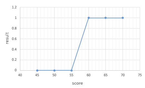
그래프는 S자 모양.
이러한 관계를 표현하기 위한 가설 : H(x) = f(Wx + b)
이때 시그모이드 함수 f를 사용한다.
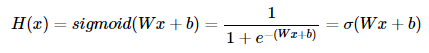
*cf) Sigmoid 함수
출력값을 0과 1 사이 값으로 조정 -> 분류 작업에 사용 가능
W값이 클 수록 경사가 커지고 W가 작아지면 경사가 작아짐.
b값에 따라 그래프가 좌,우로 이동한다.
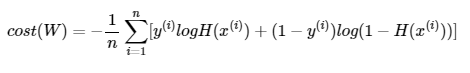
로지스틱 회귀 cost fuction
선형회귀와 같이 MSE를 사용하면 안된다. 왜? 비용함수를 미분하면 심한 비볼록 형태 그래프 나옴.
이러한 구불구불한 형태의 그래프에 경사 하강법을 사용할 경우 문제점
-> 경사 하강법이 오차가 최솟값이 되는 구간에 도착했다고 판단한 구가이 실제 오차가 최소 값이 되는 구간이 아닐 수 있음.

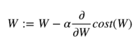
Weight update via Gradient Descent
0.
import torch
import torch.nn as nn
import torch.nn.functional as F
import torch.optim as optim

x_data = [[1, 2], [2, 3], [3, 1], [4, 3], [5, 3], [6, 2]]
y_data = [[0], [0], [0], [1], [1], [1]]
x_train = torch.FloatTensor(x_data)
y_train = torch.FloatTensor(y_data)
print(x_train.shape)
print(y_train.shape)

##################output###################

#데이터 형태 파악
torch.Size([6, 2])
torch.Size([6, 1])
1. Computing the Hypothesis
W, b 설정
W = torch.zeros((2,1), requires_grad=True)
b = torch.zeros(1, requires_grad = True)
*cf ) torch.exp()함수로 exponential function 구현 가능
hypothesis = 1 / (1+torch.exp(-(x_train.matmul(W) + b)))
파이토치에서 제공하는 torch.sigmoid 사용해서 더 간단하게 구현 가능.
hypo = torch.sigmoid(x_train.matmul(W)+b)print(hypo)
print(y_train)
##################output###################
tensor([[0.5000],
[0.5000],
[0.5000],
[0.5000],
[0.5000],
[0.5000]], grad_fn=<SigmoidBackward0>)
tensor([[0.],
[0.],
[0.],
[1.],
[1.],
[1.]])*x_train.matmul(W)+b = 시그마(x_test*W+b)
2. cost 구하기
하나의 샘플에 대해서만 오차를 구하는 식
-(y_train[0] * torch.log(hypothesis[0]) +
  (1 - y_train[0]) * torch.log(1 - hypothesis[0]))
전체에 대해서(모든 원소에 대해서) 오차의 평균 구하기
losses = -(y_train * torch.log(hypothesis) +
           (1 - y_train) * torch.log(1 - hypothesis))
cost = losses.mean()
print(cost)

##################output###################

tensor(0.6931, grad_fn=<MeanBackward0>)
하지만 이렇게 하나하나 다 구현하지 않아도 이미 pytorch에서 로지스틱 회귀 cost 함수 제공하니까 그거 사용하자...후....

식 하나하나 구현하기 너무 귀찮아요..
F.binary_cross_entropy (예측값, 실제값)
F.binary_cross_entropy(hypothesis, y_train)결과는 역시 같다. (이미 누군가가 만들어놓은거 쓰자... 삶의 질이 1000배는 올라간다)
3. 학습
optimizer = optim.SGD([W, b], lr=1)

nb_epochs = 1000
for epoch in range(nb_epochs + 1):

    # Cost 계산
    hypothesis = torch.sigmoid(x_train.matmul(W) + b)
    cost = -(y_train * torch.log(hypothesis) +
             (1 - y_train) * torch.log(1 - hypothesis)).mean()

    # cost로 H(x) 개선
    optimizer.zero_grad()
    cost.backward()
    optimizer.step()

    # 100번마다 로그 출력
    if epoch % 100 == 0:
        print('Epoch {:4d}/{} Cost: {:.6f}'.format(
            epoch, nb_epochs, cost.item()
        ))
4. 확인
한번 훈련시킨 W와 b의 값 사용해서 예측값 출력
hypothesis = torch.sigmoid(x_train.matmul(W) + b)
print(hypothesis)

##################output###################

tensor([[2.7648e-04],
        [3.1608e-02],
        [3.8977e-02],
        [9.5622e-01],
        [9.9823e-01],
        [9.9969e-01]], grad_fn=<SigmoidBackward0>)
0과 1 사이의 값을 가지고 있음.
0.5 넘으면 true, 아니면 false로 값을 정해보자.
prediction = hypothesis >= torch.FloatTensor([0.5])
print(prediction)

##################output###################

tensor([[False],
        [False],
        [False],
        [ True],
        [ True],
        [ True]])
nn.Module과 nn.Sigmoid 사용해서 구현해보기
model = nn.Sequential(
   nn.Linear(2, 1), # input_dim = 2, output_dim = 1
   nn.Sigmoid() # 출력은 시그모이드 함수를 거친다
)
nn.Sequential()은 nn.Module 층을 차례로 쌓을 수 있도록 함.
다시 말해서 Wx+b와 같은 수식과 시그모이드 함수 등과 같은 여러 함수 연결 해주는 역할.
# optimizer 설정
optimizer = optim.SGD(model.parameters(), lr=1)

nb_epochs = 1000
for epoch in range(nb_epochs + 1):

    # H(x) 계산
    hypothesis = model(x_train)

    # cost 계산
    cost = F.binary_cross_entropy(hypothesis, y_train)

    # cost로 H(x) 개선
    optimizer.zero_grad()
    cost.backward()
    optimizer.step()

    # 20번마다 로그 출력
    if epoch % 10 == 0:
        prediction = hypothesis >= torch.FloatTensor([0.5]) # 예측값이 0.5를 넘으면 True로 간주
        correct_prediction = prediction.float() == y_train # 실제값과 일치하는 경우만 True로 간주
        accuracy = correct_prediction.sum().item() / len(correct_prediction) # 정확도를 계산
        print('Epoch {:4d}/{} Cost: {:.6f} Accuracy {:2.2f}%'.format( # 각 에포크마다 정확도를 출력
            epoch, nb_epochs, cost.item(), accuracy * 100,
        ))
output을 보면 중간부터 accuracy가 100%가 나옴.
print(list(model.parameters()))

##################output###################

[Parameter containing:
tensor([[3.2534, 1.5181]], requires_grad=True), Parameter containing:
tensor([-14.4839], requires_grad=True)]
클래스로 구현하기
class BinaryClassifier(nn.Module):
    def __init__(self):
        super().__init__()
        self.linear = nn.Linear(2,1)
        self.sigmoid = nn.Sigmoid()

    def forward(self, x):
        return self.sigmoid(self.linear(x))
클래스 형태의 모델은 nn.Module을 상속받음.
__init__() 에서 모델의 구조와 동작 정의하는 생성자 정의, 객체 생성 시에 자동 호출
super()함수에서 만든 클래스는 nn.Module 클래스의 속성들 가지고 초기화.
ex) model이란 이름 객체 생성 후 model(input data)과 같이 객체 호출하면 자동으로 forward 연산 수행
model_c = BinaryClassifier()

optimizer = optim.SGD(model_c.parameters(), lr=1)

nb_epochs = 1000
for epoch in range(nb_epochs + 1):

    # H(x) 계산
    hypothesis = model_c(x_train)

    # cost 계산
    cost = F.binary_cross_entropy(hypothesis, y_train)

    # cost로 H(x) 개선
    optimizer.zero_grad()
    cost.backward()
    optimizer.step()

    # 20번마다 로그 출력
    if epoch % 10 == 0:
        prediction = hypothesis >= torch.FloatTensor([0.5]) # 예측값이 0.5를 넘으면 True로 간주
        correct_prediction = prediction.float() == y_train # 실제값과 일치하는 경우만 True로 간주
        accuracy = correct_prediction.sum().item() / len(correct_prediction) # 정확도를 계산
        print('Epoch {:4d}/{} Cost: {:.6f} Accuracy {:2.2f}%'.format( # 각 에포크마다 정확도를 출력
            epoch, nb_epochs, cost.item(), accuracy * 100,
))'Pytorch' 카테고리의 다른 글
| MNIST 분류 by softmax regression (0) | 2022.12.29 |
|---|---|
| SoftMax Regression (0) | 2022.12.29 |
| Mini Batch and Data Load (0) | 2022.12.29 |
| Linear Regression (0) | 2022.12.27 |
| Tensor manipulation (0) | 2022.12.27 |