-Each element can be accessed using index. same as normal array
Can edit elements by using index.
-Can assignment - 배정,배치
-Can copying... using copy method "copy()"
In this case, copy address value.
-Vector Equality : "==" operateor checks whether the two vectors (operand) are the same or not. And return boolean value.
On NUMPY : "==" on numpy arrays perform element-wise comparison.
-Be careful that scalar and vector are different. Especially 1-vector.
For numpy arrays, python checks elements inside the numpy array are equal to the scalar value(element-wise comparision). The specified value compares all elements of the vector.
x = 2022
y = np.array([2022,2022])
x == y
array([ True, True])
- A block vector can be created using np.concatenate()
x = np.array([1,1])
y = np.array([2,2,2])
z = np.concatenate((x,y))
print(z)
[1 1 2 2 2]*Caution : This is not a block vector. this is a list of vectors.
x = [1,1]
y = [2,2,2]
z = [x,y]
print(z)
[[1, 1], [2, 2, 2]]
- Subvector : Can slice
- Zero vector, Ones vector
- Vectors can be created using random numbers
np.random.random(4)
-Unit vector
import numpy as np
size = 4
unit_vectors = []
for i in range(size):
    v = np.zeros(size) #create zero vector
    v[i] = 1
    unit_vectors.append(v)
print(unit_vectors)
[array([1., 0., 0., 0.]), array([0., 1., 0., 0.]), array([0., 0., 1., 0.]), array([0., 0., 0., 1.])]
-Plotting
import matplotlib.pyplot as plt
data = [71,71,68,69,69,68,74,77,82,85,86,88,82,69,85,86,79,77,75,73,71,70,69,69,69,69,69,67,
       76,77,82,84,80,78,79]
plt.plot(data, '-bo')
plt.savefig("temperature.pdf" , format = 'pdf')
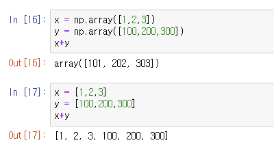
-Addition / Subtraction
also element-wise operations in numpy
x = np.array([1,2,3])
y = np.array([100,200,300])
print('x+y = ', x+y)
print('x-y = ', x-y)
x+y = [101 202 303]
x-y = [ -99 -198 -297]-"+" operator for lists in python is used for concatenation.
- Linear combination
Implement a function that
1) takes coefficients and vectors
2) returns linear combination of the input vectors
#1
x = np.array([1,2])
y = np.array([100,200])
a = 0.5
b = 0.5
c = a*x + b*y
print(c)
[ 50.5 101. ]#2
x = np.array([1,2])
y = np.array([100,200])
vectors = [x,y]
coefs = [0.5,0.5]

def linearCombination(vecs, coefs):
    res = np.zeros(len(vecs[0]))
    for i in range(len(vecs)):
        res += coefs[i]*vecs[i]
    return res
linearCombination(vectors, coefs)
array([ 50.5, 101. ])
Example
Suppose that 100-vector gives the age distribution of some population, with the number of people of age -1, for i = 1, ..., 100. How can you express the total number of people with age between 5 and 18 (inclusive)?
⇒ x6 + x7 + . . . + x19
100차원인 벡터가 있다. 이 어떠한 집단의 인구분포를 나타내는데, xi는 i-1살인 사람들의 숫자를 나타낸다. i는 1부터 100까지이다. 5살에서 18살까지의 총 인구수의 합을 어떻게 구할 것인가?
• If is given, you can calculate using the following vector
s = np.concatenate([np.zeros(5), np.ones(14), np.zeros(81)])
⇒ s @ x
step 1) 10-vector라고 가정하고 4살부터 7살까지 인구수의 합을 먼저 구해보았다.
I supposed the age distribution 10-vector first, and express the total number of people with age between 4 and 7.
size = 10
x = np.array([47,58,66,79,90,188,101,81,70,53])
s = np.concatenate([np.zeros(4), np.ones(4), np.zeros(2)])
print(s)
print(s@x)
[0. 0. 0. 0. 1. 1. 1. 1. 0. 0.]
460.0벡터의 inner product(내적) 사용했다. 처음에는 무슨 말인지 잘 감이 안잡혔는데 확실히 10차원으로 줄이니까 이해가 쉬웠다. inner product라는 용어가 낯설고 생소해서 느낌이 안 온 것 같기두.. 한글로 하면 내적임. 이러면 이해 완.이다
*A block vector can be created using np.concatenate()
위 문장을 상기시켜보자. 블록벡터는 concatenate를 사용해서 만들 수 있다. 내가 구해야하는 나이에 해당하는 요소들은 모두 원벡터로, 나머지는 영벡터로 설정한 다음에 내적을 하면 된다. 내적이 뭔지는 기억하겠지? 기억이 안 나면 바로 전 포스팅을 봐라. 쨌든 이와 같은 논리로 편하게 답을 구할 수 있다.
step 2) 위와 같은 조건에서 범위만 바꾼다면? 1살~3살 그리고 6~8살 인구 수의 총합을 구해보자
size = 10
x = np.array([47,58,66,79,90,188,101,81,70,53])
s= np.concatenate([np.zeros(1),np.ones(3),np.zeros(2),np.ones(3),np.zeros(1)])
print(s)
print(s@x)
[0. 1. 1. 1. 0. 0. 1. 1. 1. 0.]
455.0논리는 똑같다. 이제 s라는 블록벡터를 만들 때 더 쪼개주기만 하면 됨. 그리고 마지막에 np.zero() 그리고 np.ones() 괄호 안의 숫자의 총 합이 size와 같은지 체크해보자.
-Complexity
Time module can be used to estimate time-complexity
import time
a = np.random.random(10**5)
b = np.random.random(10**5)
start = time.time()
a@b
end = time.time()
print(end-start)

start = time.time()
a@b
end = time.time()
print(end-start)

start = time.time()
a@b
end = time.time()
print(end-start)
0.0009229183197021484
0.0005002021789550781
0.00020432472229003906*The result varies from time to time depending on the sys.
'Major > Linear Algebra' 카테고리의 다른 글
| Matrices,Matrix-vector multiplication,Numpy with python (0) | 2022.04.15 |
|---|---|
| K-means algorithm (0) | 2022.04.15 |
| Vector notation & operations & my proof (0) | 2022.03.03 |
